Highly Effective Genco Habit #2: Maintenance Optimization

Maintenance schedule optimization can be a full-time job, especially with a large, diverse portfolio. It’s a fluid process, and the inputs are coming from multiple sources, including the market, fuel supplies, weather forecasts, plant operations, and your own boss – just to name a few. Simulating an out-of-service unit and comparing profit results with model runs that keep that unit online provide a quantifiable basis for outage scheduling. It’s not a precise science, but it is a process that should be done very methodically. It’s also an area that regulators love to explore, so you need to have a defensible, consistent approach when taking units offline for maintenance and testing.

This article will examine a few common near-, mid-, and longer-term scenarios and how a Unit Commitment and Economic Dispatch (UC&ED) model can at least provide a consistent basis for decision-making. The basic process for each scenario is similar:

1. Begin by updating your model with the latest power and fuel prices, load forecast, deals, known de-rates and outages, initial conditions, and other relevant inputs.
2. Set up several model runs with all things held equal except the specific outage or de-rate scenarios you wish to compare.

One of your first runs will be a baseline to which you compare the total profit margin with that of the others. The scenarios may focus on when to take an outage for just one unit or may have you looking at many different units when planning a maintenance season. Regardless, it is important to collect your results in Excel or a database report, so you can rank them and clearly show how you arrived at the decision.

Near-Term Maintenance Optimization

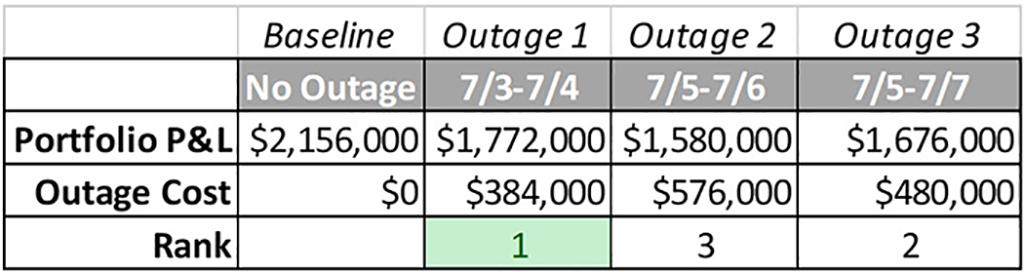
“Near-term” here is defined as being within the week. For example, one of your units just reported a tube leak but can stay online for a few days if needed. You look at the 7-Day UC schedule from this morning and see that there isn’t a great time this week to lose this unit since prices are strong. It’s not a forced outage (yet), so do we keep the unit running for a few days or shut it down now?

Below is an example of what the model output might look like. Compared to the baseline scenario with no outage, we see that, given forecasted power and fuel prices, the first window of opportunity for the 2-day outage is the best option. In exercising it, we would communicate to the plant to come offline over the long weekend and fix the issue before higher prices hit later in the week.

Mid-Term Maintenance Optimization

For our purposes, we define “mid-term” as being around 7-30 days, which generally correlates with the outer reaches of most peoples’ weather forecast “comfort zone.” Some forecast services provide 90-day outlooks, which obviously need to be taken with a few grains of salt. In this time frame, you begin to see requests for various test activities and preventative maintenance, such as:

• Hot path inspections
• Heat rate testing
• Relative Accuracy Test Audit (RATA)

The methodology here is very similar to near-term planning, but you may want to run more scenarios since there can be greater discretion about when (and if) it makes sense to take an outage. Because of increased uncertainty, you may want to test low/medium/high LMP forecast scenarios in addition to weighing the costs and likelihood of those scenarios, which makes things a bit more complex. Qualitative factors may also be considered and, if utilized, must be documented in case your plan is audited.

Long-Term Maintenance Optimization

Long-term maintenance planning is more complex for several reasons.  First, there is even more uncertainty associated with a host of factors, including prices, the available asset stack (bilaterals, renewable availability, forced outages, etc.), and weather during less predictable shoulder months.  Your long-term forecast probably reflects (typical) seasonality without attempting to predict the inevitable mid-April freeze or October tropical storm.  What also makes long-term planning more difficult is that you may be looking to take multiple outages at once, and possibly for some very large units.

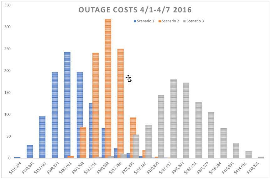
Stochastic modeling is one way to deal with increasing levels of uncertainty. The modeled output that results from using this method is not a point forecast but rather a histogram that shows a range of possibilities. After identifying the discrete scenarios for an outage season (initially considering scheduling constraints and total outage capacity limitations), you’d run the model hundreds or even thousands of times with different price paths (established from forward price, correlations, and volatility curves) and forced outages in order to assess a range of possible outputs. The more uncertainty, the wider the histogram or the larger the profit standard deviation.

Below is an example of what you might see when comparing opportunity outage costs of three scenarios during a week of the maintenance season.  Each stochastic run needs its own base case and change case to calculate the difference for each run to build the histogram of outage costs. After running all the scenarios, collect the data and award a higher rank to the lower average and lower standard deviations of costs to help guide your decision-making.

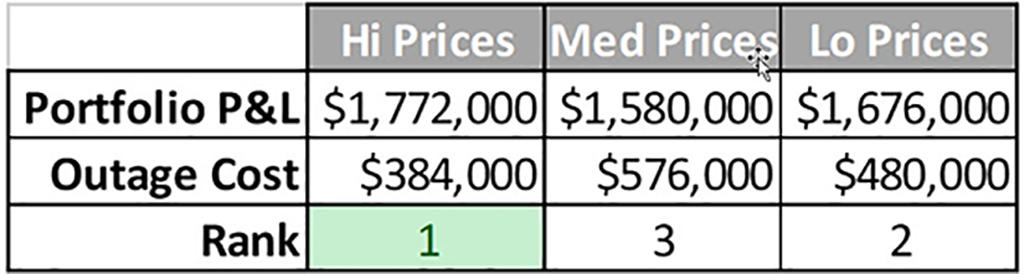
A somewhat simpler alternative to stochastic modeling incorporates high, low, and medium scenarios to get a feel for the range of possible outcomes for each outage option. Your results will depend on how you define your scenarios and the relationship between fuel and power prices. In the following example, it looks like the high price scenario for one of the outage options is actually better than the others, which may be counter-intuitive. It may be that although overall prices are higher in this scenario, the heat-rate spread narrows, making the unit less profitable during the proposed outage window. That may signal a good time to go offline compared to others.

Both of the long-term planning methods described above require more work than a deterministic (spot forecast) approach, but don’t let their complexity deter you from more deeply assessing uncertainty and placing some quantitative structure around your decisions.

Valuing Long-Term Service Agreements (LTSA) is another use case for the stochastic modeling method since the LTSA imposes penalties for exceeding annual run-time and start-up limits.  Simulation of a combined cycle generator, using various start and VOM (Variable Operations and Maintenance) costs, can determine whether the cost of an LTSA is economical.  Here, you would:

1. Input the start-up and run-time limitations detailed in the LTSA and then simulate a year of operations to compare results to other simulations using an alternative maintenance plan. 
2. Review the output to see which run generates the most profit-taking penalties. 

Alternatively, if an LTSA already exists, a stochastic model can help determine what values to use for start-up and VOM costs so that utilization is kept within contractual limits.  Use an iterative approach and vary the VOM and start-up hurdle costs in each set of simulations to arrive at the ones that, on average, yield the most profits.

Becoming a sophisticated, data-driven trading organization doesn’t happen overnight, but the journey is both interesting and rewarding for those who choose it.

Up Next…

Look for the next post in our series, “7 Habits of Highly Effective GENCOS”, that will cover the Operation and bidding of Complex Assets.

Contact Us if you have any questions for our blog authors or other subject matter experts. To automatically receive email updates when new PCI posts are published, click on the RSS icon in the top right-hand corner of any blog page and copy it into your feed.