


In many electricity markets, there is a “spot” price (or Locational Marginal Price, LMP) for power –a wholesale price that power and energy companies, industrial customers, cities, and other entities pay for power produced and consumed at this moment. This “spot” is different from the many other types of pricing used to describe the power market – concepts such as the “forward price curve,” the “day-ahead price,” the “broker price,” and many others.
In addition, most markets acknowledge that power does not flow unimpeded throughout the grid. During certain conditions, bottlenecks in the electric transmission system can make it challenging to meet demand in some regions. Markets use pricing to incentivize the generation of power in specific locations to alleviate these bottlenecks and restore the flow of electricity at safe levels.
With these two concepts in mind, “spot price” is best described as the price at which generators are willing to sell power to meet electrical demand. This price is calculated and dispatched by a central Independent System Operator minute by minute in real-time while simultaneously factoring in the physical constraints of the transmission system over which the power must flow. Inherent in this description are the two chief components of this price formation: marginal cost and transmission constraints. Let’s look at these two separately.
What is marginal cost dispatch?
In most electricity markets in the U.S., the grid operator uses an economic dispatch program to issue orders to generators to throttle up when demand rises and throttle back down when demand falls. This economic dispatch program uses a series of offer curves submitted by each resource as its input. The offer curve tells the grid operator the output level at which the resource is willing to operate based on market prices. For example:
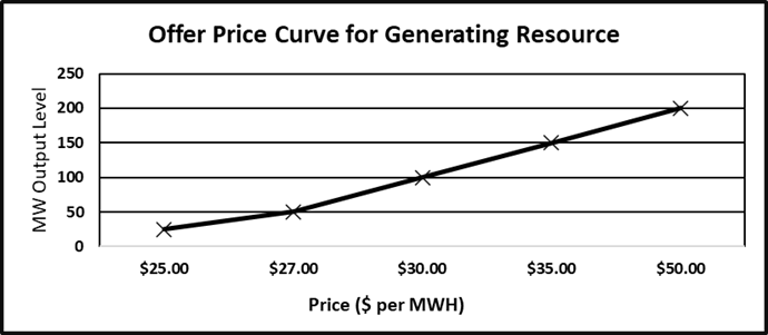
The resource is willing to generate 50 MW when the price reaches $27/MWH but will move up to 100 MW when the price rises to $30.
How are these prices set? Economic theory tells us that the offer price should be equal to the marginal cost of production. At first glimpse, this sounds dubious: How can profit be captured?
This issue can be explained by diving deeper into how the dispatch algorithm works. For every increase in power needed by the grid, the operator must select the resource with the curve that offers the lowest cost for the marginal megawatt. If the resource offers a price lower than its cost and is selected to run, it loses money. If it offers a price higher than its marginal cost, it risks not being selected at all. One must be in the game to earn revenue, but one doesn’t want to lose money, so offering a unit at its marginal cost is reasonable.*
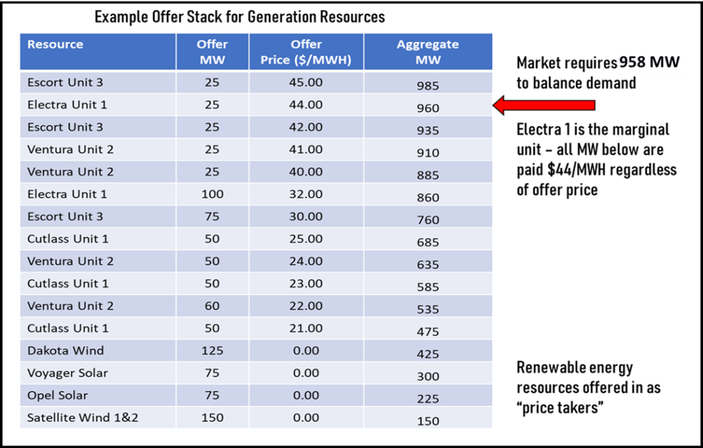
Also, when the grid operator selects the next megawatt, the price of that marginal megawatt (on that resource’s offer curve) sets the price for the entire market. This clearing price is paid to all participants for all megawatts delivered during that interval, regardless of any preceding offer curve. In the example below, the grid seeks to dispatch 958 MW during the next interval. From the stack of resource offer curves, we can see that the marginal unit is Electra Unit 1 – it is willing to sell 25 MW of power for $44/MWH, which is enough power, combined with all the lower-priced offers below it, to satisfy the demand on the system. Should one more megawatt be needed, it would come from Electra 1, at $44/MWH. This is called the Market Clearing Price (MCP).
Once the grid operator accomplishes this dispatch, all the units are electronically given their orders to throttle up or down to meet their new setpoints, but all are paid for the MCP of $44/MWH for the energy produced in that interval, regardless of their offer price.
How do transmission constraints affect pricing?
In the above example, the system is simplified and assumes any combination of the power units in the dispatch stack could satisfy demand. In actual power grids, there exist areas with either too much or too little power generation capacity, insufficient electric transmission capacity, or other factors that can constrain the free flow of power to all parts of the region. This problem can be exacerbated by transmission line outages, which change power flow patterns, or even seasonal factors such as high wind-producing periods or high load seasons. The ISO maintains a constant assessment of the transmission system’s topology, including line outages, ratings, and power generator status, and constantly updates computer models to analyze potential power flow restrictions and other problems.
The output of these computer models is combined with the marginal cost dispatch activity described above to form the Locational Marginal Price (LMP). This Security Constrained Economic Dispatch (SCED) calculates prices at each power plant, transmission substation, and other locations to accurately dispatch generators to meet the combined load of the grid without endangering any transmission system element.
Let’s see how transmission constraints affect pricing. The simplified diagram below shows that Ventura Unit 1 has the lowest marginal cost up to 100 MW, the limit of the connecting transmission line, so Locational Marginal Pricing at Townsville will remain at $25/MWH at loads below 100 MW. Dispatching Ventura 1 above 100 MW will jeopardize the security of the transmission line, so Ventura 2 is dispatched at $27/MWH for loads from 100 MW to 200 MW. The Townsville LMP is $27/MWH. Once approaching 200 MW, the transmission line from Ventura 2 to Townsville is limited, so a third source must be dispatched to meet demand at this point.
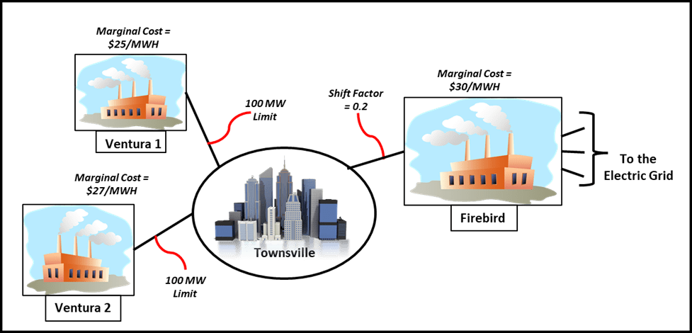
Once Townsville’s load reaches 200 MW, the incremental megawatt must come from Firebird 1, so we would assume the LMP would rise to $30/MWH. But Firebird 1 also connects to the rest of the grid, so only a portion of its output will flow to Townsville – the rest will flow elsewhere in the grid, including to serve other loads.
The ISO has modeled this environment and calculated that 20% of Firebird 1’s power will flow to Townsville. Put another way, for Firebird 1 to supply 1 megawatt to Townsville, it will have to throttle up 5 megawatts (1 ÷ 20%). Since Firebird 1’s offer curve asks for $30/MWH, we multiply this price by the “shift factor” (1 ÷ 20%), and we get a price of $150/MWH as the new Locational Marginal Pricing for the Townsville location. Ironically, at precisely 200 MW, both Ventura 1 and Ventura 2 are paid $150/MWH, but Firebird 1 is paid nothing since they produced nothing. (Please note: This simplistic description is intended for illustration only, with only one load and three generators. In an actual grid, hundreds of loads and generators all feed the same model, creating much more granularity in the dispatch. Also, SCED dispatch honors N-1 contingencies; that is, the dispatch will ensure the system’s security even if any one element is suddenly lost due to outage.)
Notes on marginal costs
The largest factor in the marginal cost is the fuel cost for thermal units. Because the marginal fuel requirement varies along a unit’s heat rate curve, the marginal cost differs for operations in the lower end of the output range versus the higher end. It is also appropriate to include variable operations and maintenance costs, as well as true consumables, in the marginal costs as well. Some companies also include an allowance to accrue against future outage costs or recover previous outage costs. In any case, accurate calculation of marginal costs is imperative for units that are likely to be on the dispatch margin in the market.
Neither renewable energy nor nuclear units are considered “marginal” units in most markets. Since there is no fuel, the marginal costs are essentially zero for renewable energy units, so many of these units are offered into the market at $0/MWH to ensure they operate at full capacity. However, should Locational Marginal Pricings dive below zero, the unit will shut down to avoid paying the grid for the privilege of generating power. Nuclear units, which are difficult or impossible to throttle, require special care in their offer strategy to ensure they are dispatched at their most efficient point (usually 100%).
Locational Marginal Pricing: what to keep in mind
This effect of integrating transmission security into the formation of locational marginal pricing does two things for the market:
- It helps determine which generators should run to meet regional demands in real-time, but in a way that avoids danger to the transmission grid.
- It provides clues to where improvement and investment should be made. For example, the significant jump in price at Townsville at 200 MW load is an incentive to invest in improvements to its transmission lines from the Ventura units, construct a new unit or other action to avoid the pain of such high prices.
The use of Locational Marginal Prices in dispatching an electric power market in real-time seeks to find the power generated at the lowest cost for the benefit of the entire system. When the transmission grid is relatively lightly loaded, there may not be congestion at all, so LMPs for all locations in the market may be the same. But as complexity is introduced in the form of line outages, high loads, rapid generation changes due to swings in wind velocities, the grid needs to respond by shifting the generation sources to locations that do not exacerbate the transmission bottlenecks. Price separation appears in different regions of the grid. Chronic high or low prices in each region provide clues as to where opportunities may exist.
Optimize your Locational Marginal Pricing strategies
Understanding and leveraging Locational Marginal Pricing (LMP) can significantly enhance your market participation and profitability. Discover how PCI’s Portfolio Optimization solutions can help you navigate LMP markets efficiently and effectively.